[논문리뷰] Score-CAM: Score-Weighted Visual Explanations for Convolutional Neural Networks

게시 2021/04/12

By JeongHwarr

8 분읽는 시간

Score-CAM: Score-Weighted Visual Explanations for Convolutional Neural Networks은 CVPR 2020에 제출된 논문이다. Gradient에 대한 의존성을 제거하여 CAM을 구한다는 특징을 가진다.

1. Gradient의 문제점

Gradient Saturation
Gradient는 sigmoid function등의 영향으로 값이 거의 소실될 수 있고, 여러 노이즈가 포함된 값이다.
False confidence

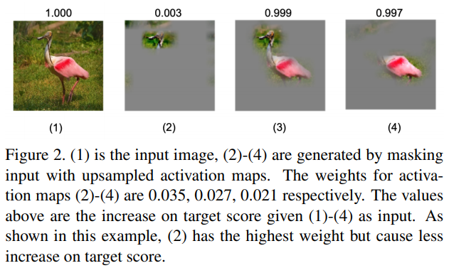
기존 CAM 방법에서는 activation map의 weight가 target score를 형성하는데에 중요한 부분일 것이라는 가정을 하였다. 하지만 위의 상황처럼 실제 그러지 않은 경우가 많다. 예를 들어 위의 (2) 이미지가 그렇다. (2)의 activation map의 weight는 0.035로 제일 높고, target score는 0.003으로 제일 낮다. 이처럼 기존 CAM의 가정과는 다르게 activation map의 weight와 target score는 비례하지 않는 경우가 많다.

2. Score-CAM

2-1. Channel-wise Increase of Confidence (CIC)

Increase of confidence는 DeepLIFT 등에서도 사용된 개념이다. 이는 베이스라인과 비교하여 주어진 입력에 대한 결과 차이를 통해 중요도를 나타내는 개념이다. 이 개념을 이용해서 저자는 아래의 식과 같은 Channel-wise Increase of Confidence를 정의하였다.

\[\tag{1}C(A^k_l)=f(X\circ{H^k_l})-f(X_b)\\ \text{where } H^k_l=s(Up(A^k_l))\]

$A^k_l$: $l$번째 $k$채널의 feature map, $X$:입력 이미지, $Up$은 업샘플링, $s$: 노멀라이징, $f$: 모델

Feature map을 업샘플링 한 후 노멀라이징하여, 입력 이미지와 point-wise manipulation을 해준다. 그 결과를 모델에 넣어서 나온 값과 원래의 베이스라인 이미지를 모델에 넣어서 나온 값을 빼서 Increase of Confidence를 구해준다. 저자는 여기서 베이스라인 이미지를 값이 모두 0인 black 이미지로 다루었고, $X_b$는 무시되어 최종적으로 $C(A^k_l)$은 아래의 식으로 된다. (이 부분은 논문에선 못 찾았던 것 같다. 저자가 구현한 코드에서 의문점이 생겨 질문했더니 그렇게 답을 받았다.)

\[\tag{2}C(A^k_l)=f(X\circ{H^k_l})\\ \text{where } H^k_l=s(Up(A^k_l))\]

2-2. Score-CAM 구하는 과정

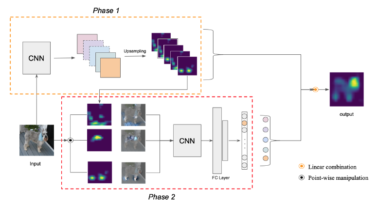
Phase 1에서 입력 이미지를 모델에 넣어 feature map를 구한다. 이 feature map은 업샘플링과 노멀라이징 과정을 거쳐 식 (2)식의 ${H^k_l}$가 된다. 이 ${H^k_l}$는 마스크처럼 생각할 수 있다.
Phase 2에서 입력 이미지와 phase 1에서 얻은 ${H^k_l}$를 point-wise manipulation한다. 이 과정에서 식 (2)의 $X\circ{H^k_l}$가 얻어진다. 이 값을 모델에 넣어 또 다른 target score인 $f(X\circ{H^k_l})$를 구한다. 최종적으로 $C(A^k_l)$가 구해진다.
Phase 1에서 구한 feature map과 phase 2에서 구한 $C(A^k_l)$ 이용하여 아래의 식으로 linear combination을 하여 Score-CAM을 구한다.

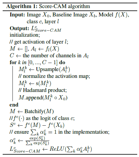
\[\tag{2}L^c_{Score-CAM}=ReLU(\sum_ka^c_kA^k_l)\\ \text{where }a^c_k=C(A^k_l)\]

전체적인 알고리즘은 아래의 과정으로 다시 표현할 수 있다.

Activation normalize는 아래의 식으로 이루어진다.

\[\tag{3}s(A^k_l)=\frac{A^k_l-\min{A^k_l}}{\max{A^k_l}-\min{A^k_l}}\]

Batchify는 메모리를 효율적으로 사용하기 위해 사용된다. Feature map을 원본 사이즈로 업샘플링하기에 메모리 공간이 많이 필요하다. 이를 나눠서 처리해주기 위한 알고리즘을 의미한다.

3. 결과

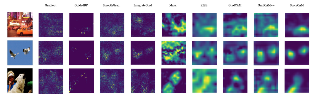
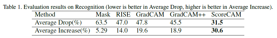
그동안의 CAM보다 recognition과 localization evaluation metric에서 더 뛰어난 성능을 보였다고 한다.

4. 코드 구현

https://github.com/haofanwang/Score-CAM: official implementation (pytorch)
https://github.com/frgfm/torch-cam/blob/565ee87b79f8fbadca70d299bb90486ab5e6ca43/torchcam/cams/cam.py#L195-L296: 여러 CAM 버전이 구현되었고, 이 안에 Score-cam도 포함되어 있다. (pytorch 버전)

저자가 구현한 ScoreCAM 코드를 통해 좀 더 자세히 이해해보자. 간단한 주석을 달아 놓았다.

  
#출처: https://github.com/haofanwang/Score-CAM/blob/master/cam/scorecam.py
def forward(self, input, class_idx=None, retain_graph=False):
        b, c, h, w = input.size() # 입력 이미지의 size 정보
        
        # predication on raw input
        logit = self.model_arch(input).cuda() # 입력 이미지에 대한 logit
        
        if class_idx is None: # target class가 주어지지 않을 때 -> 가장 확률 높은 클래스
            predicted_class = logit.max(1)[-1]
            score = logit[:, logit.max(1)[-1]].squeeze()
        else: # target class가 주어질 때 
            predicted_class = torch.LongTensor([class_idx])
            score = logit[:, class_idx].squeeze()
        
        logit = F.softmax(logit) 

        if torch.cuda.is_available(): # GPU
          predicted_class= predicted_class.cuda()
          score = score.cuda()
          logit = logit.cuda()

        self.model_arch.zero_grad()
        score.backward(retain_graph=retain_graph)
        activations = self.activations['value'] # activation map (feature map)을 가져옴
        b, k, u, v = activations.size() # activation map 사이즈 
        
        score_saliency_map = torch.zeros((1, 1, h, w)) # Masked input 

        if torch.cuda.is_available(): # GPU
          activations = activations.cuda()
          score_saliency_map = score_saliency_map.cuda()

        with torch.no_grad():
          for i in range(k): # k: 채널 개수

              # upsampling
              saliency_map = torch.unsqueeze(activations[:, i, :, :], 1)
              saliency_map = F.interpolate(saliency_map, size=(h, w), mode='bilinear', align_corners=False)
              
              if saliency_map.max() == saliency_map.min(): # Normalize 생략 조건
                continue
              
              # normalize to 0-1
              norm_saliency_map = (saliency_map - saliency_map.min()) / (saliency_map.max() - saliency_map.min())

              # how much increase if keeping the highlighted region
              # predication on masked input
              output = self.model_arch(input * norm_saliency_map)
              output = F.softmax(output)
              score = output[0][predicted_class]

              score_saliency_map +=  score * saliency_map
                
        score_saliency_map = F.relu(score_saliency_map)
        score_saliency_map_min, score_saliency_map_max = score_saliency_map.min(), score_saliency_map.max()

        if score_saliency_map_min == score_saliency_map_max:
            return None
				
				# Normalize
        score_saliency_map = (score_saliency_map - score_saliency_map_min).div(score_saliency_map_max - score_saliency_map_min).data

        return score_saliency_map

norm_saliency_map가 식(2)의 $H^k_l$를 의미한다. input * norm_saliency_map는 $f(X\circ{H^k_l})$을 의미한다. 이 값을 모델에 넣어 CIC를 얻는다. 그 CIC를 softmax 하여 원하는 클래스에 대한 score를 얻고 이 score를 각 feature map과 linear combination하고 ReLU를 취해 score_saliency_map를 얻는다. 뒤는 이렇게 해서 얻어진 score_saliency_map을 normalize하는 부분이다.

5. 느낀점

CAM을 구할 때 feature map의 weight가 실제 target score와 비례하지 않는 문제점을 해결한 아이디어란 점이 인상적이었다.. 하지만 이 알고리즘 그대로를 실제로 적용하기엔 어려움이 있다. 모든 feature map의 채널들을 입력 이미지와 같은 사이즈로 업샘플링한다는 점에서 많은 비용이 필요하다. 실제 실험에서도 계산 시간이 grad-CAM이 5초라면 Score-CAM으로는 1분 이상이 소요되었다. 메모리도 부족한 경우가 많다. CAM의 정확도도 높아졌냐고 하면 글쎄.. 실제로 적용하기 위해서는 이 아이디어를 기반으로 수정이 필요하다. 하지만 아이디어 자체는 인상적이고 좀 더 연구될 가능성이 있을 것 같다.

Review