[Tips] Optuna를 이용한 hyper parameter optimization

게시 2021/02/10

By JeongHwarr

10 분읽는 시간

이 포스트는 아래 원문의 내용을 참고하여 번역 및 수정한 것이다. 원문을 보고 싶으면 아래 링크에서 확인할 수 있다.

원문:

A 5 min guide to hyper-parameter optimization with Optuna

전체코드:

Google Colaboratory

이 게시물에서는 간단한 pytorch 신경망 훈련 스크립트를 가져와 Optuna 패키지(docs here )를 이용하여 성능을 향상 시킬 것이다.

먼저 Pytorch를 이용하여 간단한 MNIST 분류 스크립트를 짜본다. 이 스크립트를 조금 수정하여 Optuna를 이용한 이퍼 파라미터 최적화를 해본다.

1. Vanilla MNIST Classifier Framework

먼저 필요한 module을 import하고 data loader를 만드는 것으로 시작한다.

  
from __future__ import print_function
import torch
import torch.nn as nn
import torch.nn.functional as F
import torch.optim as optim
from torchvision import datasets, transforms

def get_mnist_loaders(train_batch_size, test_batch_size):
    """Get MNIST data loaders"""
    train_loader = torch.utils.data.DataLoader(
        datasets.MNIST('../data', train=True, download=True,
                       transform=transforms.Compose([
                           transforms.ToTensor(),
                           transforms.Normalize((0.1307,), (0.3081,))
                       ])),
        batch_size=train_batch_size, shuffle=True)
    
    test_loader = torch.utils.data.DataLoader(
        datasets.MNIST('../data', train=False, transform=transforms.Compose([
                           transforms.ToTensor(),
                           transforms.Normalize((0.1307,), (0.3081,))
                       ])),
        batch_size=test_batch_size, shuffle=True)

    return train_loader, test_loader

다음으로는 간단한 네트워크를 구현한다.

  
class Net(nn.Module):
    def __init__(self, activation):
        super(Net, self).__init__()
        self.conv1 = nn.Conv2d(1, 32, 3, 1)
        self.conv2 = nn.Conv2d(32, 64, 3, 1)
        self.dropout1 = nn.Dropout2d(0.25)
        self.dropout2 = nn.Dropout2d(0.5)
        self.fc1 = nn.Linear(9216, 128)
        self.fc2 = nn.Linear(128, 10)
        self.activation = activation 

    def forward(self, x):
        x = self.activation(self.conv1(x))
        x = self.conv2(x)
        x = F.max_pool2d(x, 2)
        x = self.dropout1(x)
        x = torch.flatten(x, 1)
        x = self.activation(self.fc1(x))
        x = self.dropout2(x)
        x = self.fc2(x)
        output = F.log_softmax(x, dim=1)
        return output

학습에 필요한 train 과 test 메서드를 구현한다.

  
def train(log_interval, model, train_loader, optimizer, epoch):
    model.train()
    for batch_idx, (data, target) in enumerate(train_loader):
        optimizer.zero_grad()
        output = model(data.to(device)
        loss = F.nll_loss(output, target.to(device)
        loss.backward()
        optimizer.step()
        if batch_idx % log_interval == 0:
            print('Train Epoch: {} [{}/{} ({:.0f}%)]\tLoss: {:.6f}'.format(
                epoch, batch_idx * len(data), len(train_loader.dataset),
                100. * batch_idx / len(train_loader), loss.item()))           

def test(model, test_loader):
    model.eval()
    test_loss = 0
    correct = 0
    with torch.no_grad():
        for data, target in test_loader:
            output = model(data.to(device)
            test_loss += F.nll_loss(output, target.to(device), reduction='sum').item()  # sum up batch loss
            pred = output.argmax(dim=1, keepdim=True)  # get the index of the max log-probability
            correct += pred.eq(target.to(device).view_as(pred)).sum().item()

    test_loss /= len(test_loader.dataset)
    test_accuracy = 100. * correct / len(test_loader.dataset))
    
    print('\nTest set: Average loss: {:.4f}, Accuracy: {}/{} ({:.0f}%)\n'.format(
        test_loss, correct, len(test_loader.dataset),
        100. * correct / len(test_loader.dataset)))
    
    return test_accuracy
    
   return

main 함수는 아래와 같이 구현한다. 하이퍼 파라미터는 cfg 변수 안에 선언하였다.

  
def train_mnist():
  
  cfg = { 'device' : "cuda" if torch.cuda.is_available() else "cpu",
          'train_batch_size' : 64,
          'test_batch_size' : 1000,
          'n_epochs' : 1,
          'seed' : 0,
          'log_interval' : 100,
          'save_model' : False,
          'lr' : 0.001,
          'momentum': 0.5,
          'optimizer': optim.SGD,
          'activation': F.relu}

  torch.manual_seed(cfg['seed'])
  train_loader, test_loader = get_mnist_loaders(cfg['train_batch_size'], cfg['test_batch_size'])
  model = Net(cfg['activation']).to(device)
  optimizer = cfg['optimizer'](model.parameters(), lr=cfg['lr'])
  for epoch in range(1, cfg['n_epochs'] + 1):
      train(cfg['log_interval'], model, train_loader, optimizer, epoch)
      test_accuracy = test(model, test_loader)

  if cfg['save_model']:
      torch.save(model.state_dict(), "mnist_cnn.pt")
      
  return test_accuracy

if __name__ == '__main__':
  train_mnist()

2. Enhancing the MNIST classifier framework with Optuna

Optuna 프레임워크를 아래의 명령어를 이용하여 설치한다. Optuna는 Study 개체를 기반으로 한다. 이 개체에는 필요한 파라미터 공간에 대한 정보와 sampler 방법과 pruning에 대한 모든 정보가 포함되어 있다.

pip install optuna

study은 아래의 방법으로 생성할 수 있다.

  
import optuna 
study = optuna.create_study(sampler=optuna.samplers.TPESampler(), direction='maximize')

study가 만들어진 후 search space는 trial.suggest_ 메서드를 통해 포함된다. 이것을 위에서 정의한 train_mnist 내부에 있는 config에 삽입한다. 위에서 정의한 configuration을 다음과 같이 수정한다.

  
'lr'       : 0.001,
'momentum' : 0.5,
'optimizer': optim.SGD,

  
'lr'       : trial.suggest_loguniform('lr', 1e-3, 1e-2),          
'momentum' : trial.suggest_uniform('momentum', 0.4, 0.99),
'optimizer': trial.suggest_categorical('optimizer',[optim.SGD, optim.RMSprop]),

trial에 사용할 수 있는 함수는 이 링크를 참고한다.

uniform — float values
log-uniform — float values
discrete uniform — float values with intervals
integer — integer values
categorical — categorical values from a list

만약 epoch을 설정하고 싶다면 아래의 명령어처럼 설정해주면 된다.

  
'n_epochs'       : trial.suggest_int('n_epochs', 3, 5, 1), #3~5 에폭, step은 1 

위의 방법으로 search space를 정의한 후 train_mnist() 메서드가 trial 을 입력으로 받도록 해야 한다. 따라서 train_mnist(trial) 로 바꿔준다. trial 외의 것을 입력으로 받아야 한다면 그 방법에 대해서는 해당 링크를 참조한다.

최종적으로 train_mnist 함수는 다음과 같이 될 것이다.

  
def train_mnist(trial):
  
  cfg = { 'device' : "cuda" if torch.cuda.is_available() else "cpu",
          'train_batch_size' : 64,
          'test_batch_size' : 1000,
					'n_epochs' : trial.suggest_int('n_epochs', 3, 5, 1),
          'seed' : 0,
          'log_interval' : 100,
          'save_model' : False,
					'lr' : trial.suggest_loguniform('lr', 1e-3, 1e-2),  
					'momentum' : trial.suggest_uniform('momentum', 0.4, 0.99),
					'optimizer': trial.suggest_categorical('optimizer',[optim.SGD, optim.RMSprop]),
          'activation': F.relu}

  torch.manual_seed(cfg['seed'])
  train_loader, test_loader = get_mnist_loaders(cfg['train_batch_size'], cfg['test_batch_size'])
  model = Net(cfg['activation']).to(device)
  optimizer = cfg['optimizer'](model.parameters(), lr=cfg['lr'])
  for epoch in range(1, cfg['n_epochs'] + 1):
      train(cfg['log_interval'], model, train_loader, optimizer, epoch)
      test_accuracy = test(model, test_loader)

  if cfg['save_model']:
      torch.save(model.state_dict(), "mnist_cnn.pt")
      
  return test_accuracy

3. Optimization

마지막 단계로 최적화 될 objective function을 정의한다. 이 포스트의 경우는 train_mnist 를 objective function으로 정하였고, 그 결과인 test error를 최적화 하도록 한다.

따라서, study.optimized 안에 train_mnist 함수를 파라미터로 넣어준다.

  
study.optimize(train_mnist, n_trials=20, direction='maximize')
joblib.dump(study, '/content/gdrive/My Drive/Colab_Data/studies/mnist_optuna.pkl')

train_mnist() 를 호출하기 위한 전체적인 main 코드는 다음과 같이 된다.

  
sampler = optuna.samplers.TPESampler()
      
study = optuna.create_study(sampler=sampler)
study.optimize(train_mnist, n_trials=20, direction='maximize')
joblib.dump(study, '/content/gdrive/My Drive/Colab_Data/studies/mnist_optuna.pkl')

위의 라인이 코드에 추가되면 optimizer는 샘플러에 따라 (예시에서는 TPESampler) 정의 된 매개 변수 공간을 샘플링한다.

최적화가 완료된 후 결과는 다음을 통해 데이터 프레임으로 액세스 할 수 있다 study.trials_dataframe :

  
from sklearn.externals import joblib
study = joblib.load('/content/gdrive/My Drive/Colab_Data/studies/mnist_optuna.pkl')
df = study.trials_dataframe().drop(['state','datetime_start','datetime_complete','system_attrs'], axis=1)
df.head(3)

그러면 다음과 같은 결과가 출력될 것이다.

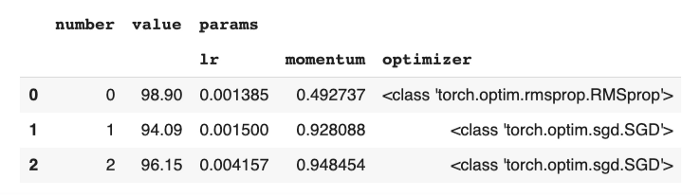
최적의 파라미터를 확인하기 위해서 study.best_trial및 study.best_params도 사용할 수 있다.

위의 방법으로 최적화를 한 후에 동일한 양의 학습 데이터와 동일한 시간으로 98.9 % 테스트 오류 (~ 6 % 개선) 결과를 얻을 수 있었다.

4. Visualization

최적의 파라미터를 찾는 것 외에도 Optuna를 통해 시각화 할 수 있다. 모든 시각화 툴은optuna.visualization 에 포함되어 있다.

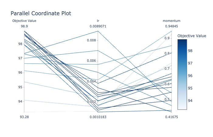
예를 들어 파라미터 간의 관계를 확인하기 위해 plot_parallel_coordinates(study) 이라는 명령어를 사용하여 아래와 같은 결과를 얻을 수 있다. (이 예시에서는 lr과 momentum이 파라미터)

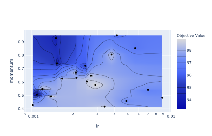
다른 방법으로 contour plot을 이용할 수도 있다. 이 결과는 plot_contour(study) 를 통해 얻을 수 있다.

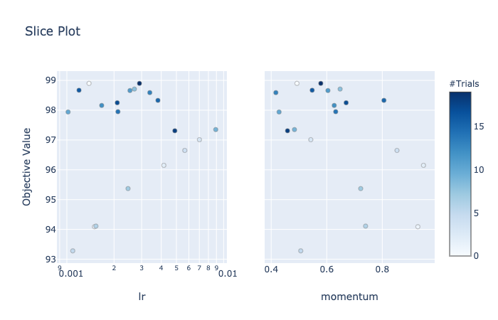
또한 slice_plot(study) 을 호출하여 slice plot을 만들 수 있다. 이는 각 파라미터에 대해 개별적인 최적의 부분 공간이 어디에 위치하는지 이해하는 데 도움이 될 수 있다.

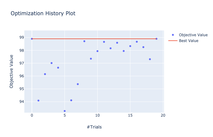
마지막으로 study history를 시각화 하기 위해 plot_optimization_history(study) 을 이용할 수도 있다.

5. 요약

실제 학습에 사용되는 함수를 수정한다. (예시에서 train_mnist 함수가 이에 해당한다. ) 이 함수는 아래의 조건을 충족해야 한다.
- 평가 지표가 될 점수를 return 해야 한다. 이 함수 안에서 모델의 파라미터를 정해준다. (trial.suggest_.. 함수 이용)
- 이 함수는 trial을 매개변수로 받아야 한다.
study.optimize 를 실행한다. 1에서 정의한 함수를 파라미터로 넘겨준다. 예시: study.optimize(train_mnist, n_trials=20, direction='maximize')

6. 참고

[1] https://towardsdatascience.com/how-to-make-your-model-awesome-with-optuna-b56d490368af

[2] https://optuna.readthedocs.io/en/stable/index.html

Tips